PDF version

3 METHODS

3.1 Source data

Table 1 lists the completed international and national regional geochemical mapping projects that were used in the compilation of the Geochemical Atlas of Northern Europe. Altogether, 28 projects, including 8 large international projects of regional and global geochemical mapping, completed in 1980-2005 (Fig. 7.), and 20 national projects (Fig. 8.) were included in this work. The national projects included 8 projects that were carried out for the composition of national geochemical atlases in Scandinavian and Baltic countries and 12 regional geochemical mapping projects from Russia. The total area covered by these regional mapping projects is 2,175,000 km² and includes Fennoscandian countries (Norway, Sweden and Finland), Baltic countries (Estonia, Latvia and Lithuania) and NW Russia. The Russian part of the project extends over 948,000 km² and covers the Republic of Karelia, the Murmansk, Arkhangelsk and Leningrad regions and parts of Pskov, Novgorod and Vologda regions.

3.2 Methods of investigation

All primary data derived from different sources had a very complex and heterogeneous structure. The data included different forms of metadata from the accomplished projects and field documentation with dissimilar descriptions of natural conditions, sample media, sampling sites and methods of sampling. The primary analytical data were incomparable because of differences in sample preparation, extraction methods and devices for measuring element concentrations. Non-uniformly scaled cartographic materials indicating the position of sampling sites and information about natural conditions were prepared in different geographical projections. Thus, further data processing was only possible after the composition of a common integrated database, providing systematization and storage of information in a unified form. Therefore, all spatial information was assigned a common coordinate system, and the documentation of different projects was coordinated with cartographic materials. Element concentration data from different projects were also transformed to single orders of concentrations.

Finally, an integrated database was created for the systematic storage of collected data. The structure of the database supports a complex approach to data processing and interpretation and also enables remote users to gain access to these data.

3.2.1 Integrated database

The integrated database includes three interrelated blocks:

• Metadata of the project. It contains a general description of every accomplished geochemical project stored in the integrated database. Information about the study area, applied methods and other details of the work is stored in a formalized form, including descriptions of the studied sample media, methods of sampling, sample preparation and analytical methods. Information about the owners of the data, storage of the original data and its availability is also included.
• Database of the project. It contains the primary analytical data in a unified form with references to analytical and field methods and coordinates of the sampling sites. A detailed description of the analytical data used for generalization of the project data is presented in Table 2. Data from 58,311 samples including 9 different sample media used in the geochemical mapping projects are stored in the database. Analytical data include concentrations of more than 60 elements and other parameters. More than 10 different analytical methods were used, including the determination of element concentrations after total, strong acid or weak acid extraction. Detection limits for each element and method are included. In the final stage the data were generalized, levelled and normalized between various projects. These new calculated values were imported to the database and were used for preparing geochemical maps. The multi-user remote mode of the work included access and interchange of information between the project group members from different institutes and countries via the Internet.
• 3. Digital cartographic information. It includes a set of specially prepared accessory maps, characterizing natural and anthropogenic features of the study area. This set of maps was used for a review of collected data and interpretation of compiled geochemical maps in their different phases. Maps were prepared at the scale 1:5,000,000 and they describe:
• natural landscape and climate conditions (including separate digital cartographic layers for soil types, large structural tectonic blocks, Quaternary deposits, vegetation zones and climate conditions);
• descriptions of the distribution of various of human activities;
• geological formations and metallogenic features of the study area (including separate digital layers of generalized geology, the scheme of the location and a catalogue of the main ore deposits with their classification in accordance with ore formation types.

The composition of this digital cartographic information was mainly based on various published works (Ahti et al. 1968, Koistinen et al. 2001, Sigmond 2002, Ignatenko 1979, Isachenko and Lavrenco 1974, Nauka 1980, Kaurichev and Gromyko 1974, Rassmusen et al. 1989, Reimann et al. 1998, Salminen et al. 2004), and only minor additions were made by this project.

3.2.2 Analytical work

New analyses were carried out at the Central Chemical Laboratory (CCHL) of VSEGEI (St.-Petersburg). Altogether, 873 mineral stream sediment samples and 63 mineral soil samples from the C-horizon collected in 2000-2001 from NW Russia were analyzed after total extraction by ICP-AES and ICP-MS. The soil samples had been analyzed earlier at the Geological Survey of Finland (GTK) laboratories and these data were used for quality assurance.

Comparison of analytical methods used at CCHL of VSEGEI and the GTK Laboratory was conducted for 39 elements: Al, Ca, Fe, K, Li, Mg, Mn, Na, Cr, Cu, Ni, V, Ti, La, Sc, Y and P (ICP-AES), and Be, Co, Zn, Ga, As, Rb, Sr, Zr, Nb, Ag, Mo, Cd, Sn, Sb, Cs, Ba, Ce, Tl, Pb, Bi, Th and U (ICP-MS). Systematic variance of concentrations for most of analyzed elements was not significant (relative systematic error was 0.9-1.1). For a small number of elements (Li, Cd, Mo, Ni, Th, and U) the data from CCHL of VSEGEI were slightly overrated, but by no more than a factor of 1.2-1.3. Considerable systematic variance was only marked for As (analytical results from CCHL of VSEGEI were 1.7 times higher). The detection limits for all elements were the same in both laboratories.

3.2.3 Data processing

Data processing started by estimating the comparability of analytical data from the various projects. In the next phase the data from these projects were levelled. After statistical processing of the levelled values, maps of the spatial distribution of separate elements were compiled. In the last phase, maps of element associations and anomalous geochemical fields were prepared.

Because of the diversity of the data, caused by differences in sampling and analytical methods, the composition of summary geochemical maps was challenging, especially taking into account the large territory with complex geology and the large variety of natural and anthropogenic landscapes. Therefore, in the first stage any significant systematic variability was minimized and respective corrections to primary analytical data were performed in order to obtain comparable background levels for actual or relative element concentrations.

Comparison of primary analytical data

Levelling of data from various sub projects was separately carried out for each of the sample media and was based on pairs of closely located samples selected from overlapping project areas. The data from the Barents Ecogeochemistry project (Salminen et al. 2004) were selected as the baseline because they regionally overlap with most of the other sub projects. Thus, the correction coefficients were calculated for various sub-project data in relation to the data of the Barents Ecogeochemistry project.

Relative systematic and random errors were calculated for every pair of element concentrations in following sequence:

• ratios of the concentration for each element i in comparison pairs (C1,i/C2,i) were calculated;
• relative systematic deviation was identified as the median value Δ_syst.= Me (50% value of the cumulative curve of these ratios);
• according to David (1977), the interval between 50% and 84.1% percentiles of the cumulative curve is equal to the standard deviation. Therefore, the 84.1% value (t_84.1%) of these ratios was taken from the cumulative curve;
• relative random divergence was calculated as ε_diverg. = t_84.1% /Me;
• relative standard error was estimated as ε = ε_diverg. √ 2 (it is assumed that the true element concentration lies between a comparable pair of uniformly precise analyses).

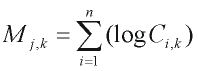
The results of the comparison of calculated parameters for relative systematic and random errors are presented in Appendix A (Tables A.1-A.7), including information on analytical methods, detection limits of elements and values of correction coefficients for corresponding pairs of compared sub-projects.

Comparison of all collected primary data and calculation of correction coefficients was carried out for moss, the organic soil horizon, mineral soil C-horizon (both total concentration and aqua regia leaching), stream and lake water and mineral stream sediment on the Russian side of the project area. Because of the lack of sufficient overlapping, significant differences in the methods of sampling, sample preparation (grain size fraction for analysis) and analytical methods used (partial leaching or determination of total content) for the sub-project data, no comparison was carried out for the upper layer of the soil and the fine fraction of till and for mineral stream sediment outside Russia. Only normalizing of the primary data was used for these data in order to prepare maps of spatial element distribution.

Normalizing of primary analytical data

The production of maps showing the spatial distribution of element concentrations and their associations required normalization of the primary analytical data from the different sub-projects. The normalization of element concentrations was performed against background values calculated as geometric means of elements concentrations for different taxons of natural landscapes. If the correction coefficients were used for the primary data, the background values were calculated for a particular group of sub-projects; for other data, background values were calculated for each sub-project separately. The values of normalized data are presented in Appendix B.

For each separate data set, calculation of the geometric mean values of element concentrations was performed sequentially according to the following formulae:

(logCi)_a.m. = (ΣlogCi,j)/n,

Ci_g.m. = 10^(logCi)_a.m.

where:

• (logCi)a.m. is the arithmetic mean of the decimal logarithm for the concentration of element i,
• Ci,j the concentration of element i in sample j,
• n the number of samples, and
• Cig.m. the geometric mean of concentrations of element i.

Maps of the spatial distribution of element concentrations and their associations

The levelled and normalized analytical data were used in drawing composite maps of the spatial distribution of element concentrations and their associations in different natural media at the scale of 1:5,000,000. In the next stage, maps of anomalous geochemical fields (AGF maps), a map of ore-bearing geochemical anomalies and an ecogeochemical map were prepared to the same scale.

ArcInfo software was used in drawing the maps. A special add-in module to ArcView Spatial Analyst, prepared by SC Mineral for data processing in the Barents Ecogeochemistry project, was applied in the map processing. This module enables

• the selection and use of any colours or symbols needed in drawing the map;
• the calculation of different statistical parameters and drawing of histograms and accumulative diagrams of parameters; and
• the selection, loading and display of accessory digital maps for the combined interpretation of the analytical data.

The software enabled rapid and efficient data processing in the preparation and production of a large number of maps included in the Atlas. Geochemical information is presented on the maps in two ways: (i) the sampling site and element concentration are presented as circles; the location of the circle shows the sampling site and the size is proportional to the concentration level; (ii) the spatial distribution of the element concentration is shown as a coloured surface based on interpolated data.

All element maps were prepared with following drawing parameters:

• The unit of the true element concentration is mg/kg for moss, the organic soil layer, the mineral soil C-horizon, stream sediment and till, and µg/l for samples of stream and lake water.
• The normalized element data is in relative units.
• Calculations of multiplicative or additive values (in relative units) for element association maps were performed according to the following formulae:
  • for true element concentration

    

    where:

    • M_j,k is the calculated value of element association j in sample k,
    • Ci, k is the concentraion of element i in sample k, and
    • n is the number of elements in association j;
  • for normalized element data

    

    where:

    • M_j,k is the calculated value of element association j in sample k,
    • C_{norm, i, k} is the normalized concentration of element i in sample k, and
    • n is the number of elements in association j.
• For drawing colour surfaces on maps the following parameters of interpolation were used:
  • the interpolation grid cell was 2,500 x 2,500 m,
  • the number of adjoining points was 8,
• smoothing was done using inverse distance weigthted interpolation (IDW) with parameter e¹.
• The legend for element concentrations and related values on both symbol and colour surface maps is divided according to percentiles.
• Each map is accompanied by a histogram and an accumulative diagram on a logarithmic scale.
• The calculated interpolation grids were masked in order to show areas with no data. This was done by buffering, and the diameter of the buffering cells was 50 km for the single-element maps and 30 km for the maps illustrating element associations.

Preparation of maps of particular and integrated anomalous geochemical fields (AGF)

The maps of anomalous geochemical fields (AGF), which show the anomaly patterns of element concentrations, were based on the data from minerogenic samples of the soil C-horizon (total and aqua regia leachable concentration of the <2 mm fraction), the fine fraction of till, stream sediments, and lake and stream water. These media primarily reflect geological and minerogenic features of the study area.

Maps comprising information on the distribution of different element associations were prepared, defining a particular association by factor analysis of the normalized element concentrations (principal components analysis, varimax rotation). The media and element associations used for preparing particular AGF maps are listed in Table 3. In map drawing a common legend based on a colour scale was used, where anomalous levels were defined according to the percentiles (Table 4).

Table 3
Table 4

In the next phase, the legends used for particular AGF maps were transferred to a common unified form (Table 5). This reclassified legend was used for drawing integrated AGF maps, which summarize results by combining both particular AGF maps for various element associations and AGF maps of different sampling media.

Calculation of all integrated AGF maps was carried out in accordance with the condition

(Ki>Kj).con(Ki,Kj),

where: Ki and Kj are values of reclassified codes for maps i and j.

According to this condition, in summarizing particular maps every anomalous geochemical field with a greater value of the code (or anomalous level) was moved to the integrated AGF map. The prepared integrated AGF maps are listed in (Table 6). As an example, map M1all_an is presented in Figure 9

3.2.4 Assessment of environment status and mineral potential of the study area

As a final result of the processing of geochemical information, an ecogeochemical map and map of ore-related geochemical anomalies, both at the scale 1:5,000,000, were prepared. This work was based on a joint interpretation of all produced cartographic material.

Ecogeochemical map

The ecogeochemical map was composed with the help of the Federal State Unitary Enterprise “IMGRE” and according to the requirements of existing Russian instructions, recommendations and legislation (IMGRE 1999, IMGRE 2001) concerning the presentation of materials with an ecogeochemical content. The map contains environmental information, including characteristic features of natural landscapes, the degree of degradation, intensity of anthropogenic influence, features of human activity and assessment of environmental status. It shows the distribution of unsatisfactory conditions in the study area.

Map of ore-related geochemical anomalies

The map of ore-related geochemical anomalies, prepared with methodological participation of FSUI “IMGRE”, shows the main results of the data interpretation and prognostic estimation of ore-related anomalous geochemical fields. These AGFs show many known ore-related anomalies, but they also show new anomalies promising for mineral exploration.

Geochemical anomalies in the areas of known or expected ore districts were contoured on the basis of the integrated AGF maps. The identified and expected ore-related districts were then combined into larger zones taking into account the geochemical and metallogenic features and the geological conditions in the areas of AGFs. The technology used in preparing the map of ore-related geochemical anomalies included the following actions:

• composition of the generalized geological map;
• tectonic zoning of the study area;
• location of ore-related and potentially ore-related AGFs;
• calculation of the parameters of each AGF;
• determination of the ore formations belonging to an AGF;
• estimation of the value of an AGF for mineral exploration;
• preparation of a catalogue of AGFs and areas promising from the point of view of mineral exploration.

The map of ore-related geochemical anomalies and its legend consists of information blocks, including the characteristics of ore-bearing and potentially ore-bearing geological complexes situated within anomalies, and scheme of the concept for metallogenic zoning of the area. An independent block consists of discovered AGFs in a rank of ore districts and their grouping into large geochemical zones, conditioning the main metallogenic features of the region. Detailed characteristics of AGFs with a description of indicator elements, typification of AGF areas according to types of known and prognostic mineral wealth, and estimation of their potential value are presented in the catalogue of the AGFs.

PDF version